Tessellated Terrain Rendering with Dynamic LOD
This report was for a project/presentation assignment for my Computer Graphics course in the Fall 2014 semester. The source code is available on BitBucket. Enjoy!
Goals and Motivation
Rendering large, detailed terrain meshes is an important issue in many graphics applications such as video games, simulators (flight, space, auto, world, etc.), and geographic information systems. The goal, as with many real-time rendering applications, is to render a high level of detail (LOD) without sacrificing efficiency and performance. The goal of this project was to explore some basic concepts for using tessellation with GPU acceleration to render large terrains in such a manner.
Some basic foundation knowledge needed to be addressed first, such as understanding the OpenGL programmable pipeline (hardware tessellation is only available in “modern” OpenGL pipelines that run programmable shaders). The role and usage of tessellation shaders and how to control the tessellation stage to dynamically alter the level of detail being rendered was next to be understood. Finally, basic concepts for terrain data structures and rendering were evaluated.
This report will look at the basics on the OpenGL 4.x programmable pipeline, the role of the tessellation engine in this pipeline, two approaches to dynamic level-of-detail using tessellation, and two basic approaches for a terrain rendering layout.
Two main resources for the project were used (many other references were consulted, of course; these two were the primary motivators). The NVIDIA whitepaper DirectX 11 Terrain Tessellation [1] serves as the main reference and motivation for the terrain rendering approaches in this project. The OpenGL 4 Shading Language Cookbook [2] was an invaluable resource when learning about the OpenGL programmable pipeline and the OpenGL Shading Language. It also provides great information about the tessellation engine in OpenGL.
OpenGL Programmable Pipeline
Previous versions of OpenGL (before version 2.0) were considered a “fixed-function” graphics pipeline [2]. Different rendering algorithms were fixed into the GPU and were simply configured through the API functions. As the API grew, more flexibility in how the graphics hardware got utilized was desired – a desire fulfilled in the development of shaders. Shaders are programs that are executed by the GPU hardware at some stage in the programmable pipeline. OpenGL shaders are written using the OpenGL Shading Language (GLSL). These programs give control over the GPU hardware for different stages of the rendering pipeline and allow developers to implement rendering algorithms in whatever way they see fit.
Although knowledge of the programmable pipeline was vital for this project, a detailed description of the pipeline is beyond the scope of this report – the focus here deals more with how the tessellation engine operates. See the “Rendering Pipeline Overview” article in the OpenGL Wiki [3] for details about the OpenGL programmable Pipeline.
OpenGL Tessellation Engine
The tessellation engine was introduced in OpenGL version 4.0 [4]. The role of the tessellation engine is to generate additional primitives on the GPU to be manipulated and rasterized given some kind of input. For terrain rendering, it would be nice to leverage this functionality by providing a smaller set of input primitives and allowing OpenGL to tessellate the interior of these input primitives to generate a larger number of output primitives efficiently.
OpenGL’s tessellation engine introduces three new components to the OpenGL pipeline: the tessellation control shader (TCS), the tessellation primitive generator (TPG), and the tessellation evaluation shader (TES). Figure 1 provides an overview of how these new components fit into the OpenGL pipeline.
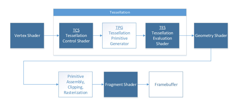
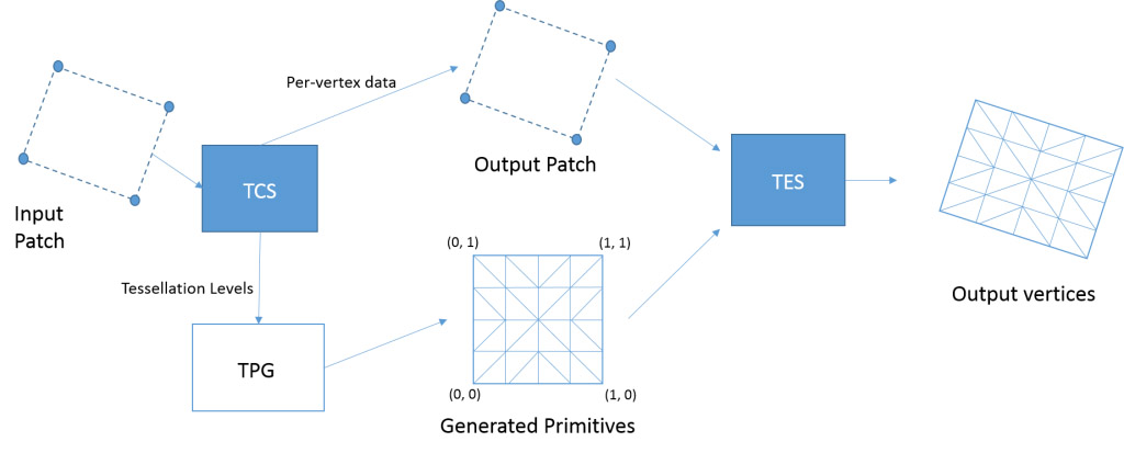
Input primitives in the form of patches (which will be explained momentarily) are fed into the tessellation engine when in use. Both the control shader (TCS) and evaluation shader (TES) are programmable stages of the pipeline; the primitive generator (TPG) is a fixed stage, but is configured through both the TCS and TES. The final output from the tessellation engine is passed along to be processed by the rest of the pipeline. Figure 2 provides a diagram of the interaction between the different stages inside the tessellation engine, which will be described next.
Tessellation Primitive Generator (TPG)
The TPG is the fixed stage of the tessellation engine and is responsible for actually generating the new primitives. It is not programmable, but it is configurable in how it will perform the tessellation [2]. The TPG is actually situated between the two programmable stages of the engine; however, its configuration is provided by both stages. The TCS determines the amount of tessellation to be performed and the TES specifies the type of primitive being tessellated (thus how to tessellate the new primitives inside the input).
When using the tessellation engine in OpenGL, the only primitive type that can be rendered by the OpenGL program are patches (GL_PATCHES) [2]. Patches are arbitrary collections of geometry, used for whatever purposes the developer wants. The number of vertices in a patch can be defined as well, up to a maximum limit imposed by OpenGL.
While input patches are arbitrary, tessellation depends on how vertices of the input patch are interpreted by the primitive generator. There are three types of primitives that the primitive generator can tessellate: isolines, triangles, and quads. The type of primitive is defined by the input expected in the evaluation shader [5]. When triangles is specified by the TES, the TPG will use barycentric interpolation to distribute the vertices of the new primitives across the inside of the input patch. If quads is specified, linear interpolation will be used [6].
Tessellation Control Shader (TCS)
The TCS is the first stage in the tessellation engine; the input patch comes from the vertex shader into the TCS. The TCS is executed once per vertex of the input patch. Its primary function is to define the tessellation levels to be used by the primitive generator – essentially asking, “How many primitives should be generated inside this patch?”
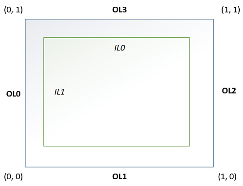
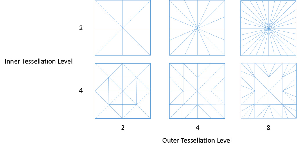
Tessellation levels are defined by two output variables in the TCS: gl_TessLevelOuter and gl_TessLevelInner [4]. These parameters will have different meanings depending on the type of primitive being tessellated. For this project, we focus on the use of quads. Figure 3 shows the different tessellation level parameters and the edges of the quad they are associated with. There are four OL parameters (outer level) and two IL parameters (inner level). Each parameter instructs the TPG how many segments to subdivide the edge into. An example of different combinations of inner and outer level configurations can be seen in Figure 4.
It is important to note that the TCS has control of both inner and outer tessellation levels and each of the six different parameters can have different tessellation levels. This is important for matching edge vertices of neighboring patches in terrain rendering to prevent cracks (as will be seen later).
Tessellation Evaluation Shader (TES)
The newly generated primitives from the TPG and the original input patch are combined into the output patch. This is fed into the TES. The TES is executed once for each vertex in the tessellated output patch (so, for each original input vertex plus all the vertices generated by the TPG). Each vertex is given a parameter-space coordinate, dependent upon what type of primitive is specified as input to the TES that is being used for tessellation. For example, quads will have a simple, normalized (u,v) coordinate pair (see Figure 3). This way the evaluation shader can manipulate the newly created vertices of the generated primitives in whatever way the programmer sees fit.
Dynamic Level of Detail
Equipped with an understanding of the tessellation engine, the goal is to vary the tessellation levels depending on how close or how far away an object (or part of the terrain) is from the camera. A portion of terrain closer to the camera will require a greater number of primitives to achieve an acceptable level of detail than will a portion of terrain farther away from the camera. The tessellation control shader is in charge of determining the tessellation levels used, so this is a good spot to implement some kind of dynamic level of detail algorithm.
This report looks at two algorithms. The first is a basic approach (referred to here as the “camera distance approach”) outlined in the OpenGL 4 Shading Language Cookbook [2] by David Wolff. The second (referred to here as the “sphere approach”) is given in DirectX11 Terrain Tessellation [1] by Iain Cantlay.
These algorithms are surprisingly simple and fairly straightforward to implement.
Camera Distance Approach
For each edge of the input patch, a calculation is performed to determine how far the edge is from the camera. This is done in the TCS. For each edge, the two vertices of the edge are projected into camera space. The distance from the camera to each vertex is calculated, then averaged. This serves as the distance to that edge.
This distance can be used to determine an appropriate outer tessellation level for the corresponding quad edge. A minimum distance and maximum distance can be set to help interpolate between the minimum available tessellation level and the maximum available level. In the case of OpenGL, the maximum tessellation level is 64 [6].
This process is done for all four edges of the quad, and the calculated tessellation level applied to the corresponding outer-level (OL) parameter. The inner tessellation levels are simply an average of the outer levels.
Sphere Approach
This algorithm attempts to tessellate based upon a target triangle size. A target triangle size is a desired width, in pixels, of any rasterized triangle on the screen with the goal being to have all triangles be as close to the same size as possible.
Each edge of the input patch is processed separately, as with the previous approach. A conceptual, invisible sphere is fit around each edge. This sphere is projected into screen space. The diameter of the sphere is then calculated. This provides a width, in pixels, that the sphere occupies on the screen. This width can be compared to the target triangle width and an appropriate tessellation level assigned. If the width is greater than the target width, the edge can be tessellated to try to match the target as closely as possible. If the width is less than the target width, there is no need to tessellate as the edge is already at or below the target width. Figure 5 illustrates the sphere approach concept.
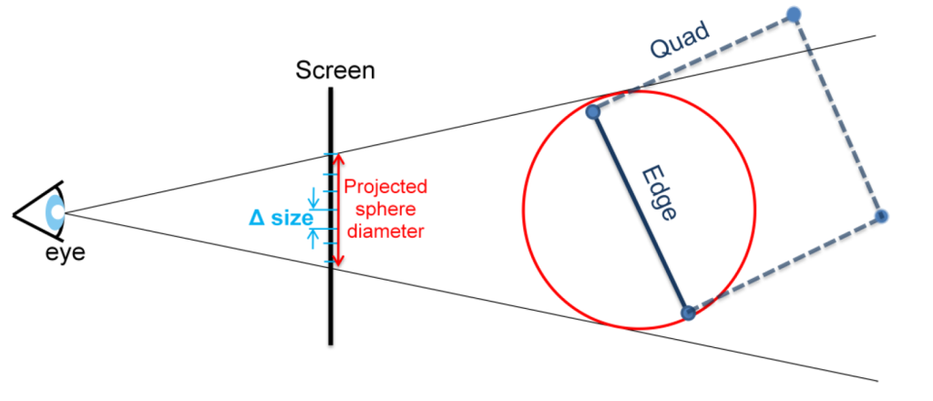
One may wonder, “Why bother with the sphere in the first place and not just map the edge directly to the screen?” This can cause problems when an edge is close or at perpendicular to the camera. The edge may actually be close physically to the camera, but when mapped to the screen, its footprint width is small, leading to an incorrect tessellation level and undesirable artifacts.
Terrain Rendering
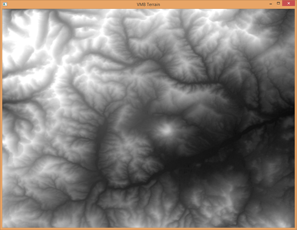
Using the foundation of tessellation and dynamic level of detail, it is time to apply these techniques to rendering terrain. A basic (non-tessellated) approach to terrain rendering is to create a large flat mesh, comprised of many vertices. A heightmap is created to define the shape of the terrain. A heightmap is an image in which each pixel represents a height value depending on the color intensity of the pixel. The heightmap can be overlaid against the terrain mesh and each vertex in the mesh sampled on heightmap to determine its height. Every vertex in the mesh then has its height offset accordingly, creating the final terrain.
As a terrain becomes larger and more complex, the number of vertices required to achieve an acceptable level of detail begins to grow. As vertices grow, performance decreases. This is where tessellation and dynamic LOD algorithms can be applied. Instead of feeding the GPU a large number of vertices, a smaller initial set of vertices can suffice with the GPU generating the required amount of additional primitives on the fly.
There are two basic approaches this report will look at, both of which are outlined in the DirectX 11 Terrain Tessellation whitepaper [1]: uniform and non-uniform patch terrains.
Uniform Patch Terrains
This approach is a simple extension of the basic terrain rendering approach mentioned earlier, except with tessellation. A grid of square patches (four vertices per patch) is created to cover a desired amount of terrain. These patches are passed into the GPU to be tessellated. The heightmap for the terrain is mapped across the entire grid of vertices. Inside the TCS, a dynamic LOD algorithm is applied. In the TES, after tessellation has been performed on the patch, each vertex samples the heightmap for the appropriate location and offsets its height accordingly.
This approach is very simple, and works to a degree. There are a couple main problems. The first is that it does not scale. As the terrain size grows, the number of input vertices keeps growing steadily along with it.
The second problem stems from the fact that there is a tessellation limit for the GPU. For terrain patches that are close to the camera, a high tessellation level is desired to achieve a high level of detail. The size of the input patch can be chosen so that, at a maximum tessellation level, the patch is tessellated enough to provide the desired level of detail when the patch is close to the camera. However, this same patch size is used throughout the entire terrain. Patches that are far away from the camera begin to converge into single pixels after perspective transforms are taken into consideration. Even at the minimum tessellation level, there could be multiple primitives being rasterized that only account for a single output pixel. This is wasteful, and leads to performance issues.
Non-Uniform Patch Terrains
To counter the limitations of tessellation levels and performance issues, terrains comprised of non-uniform patches are introduced. Patches that are close to the camera can have smaller size, allowing for acceptable levels of detail within the limited tessellation range. Patches farther from the camera are larger in size, allowing for acceptable levels of detail without an unnecessary amount of vertices.
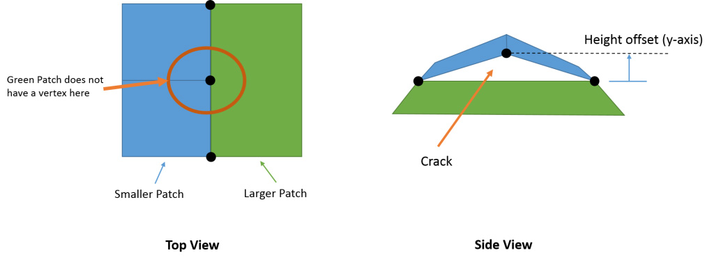
While the non-uniform approach fixes some issues, it introduces a major new problem – cracks. Since the patches are not all the same size, vertices that lie along an edge of a patch are not guaranteed to line up with the vertices of a neighboring patch of a different size. The dynamic LOD algorithm will still calculate the same tessellation level for each edge (they are in the same position, after all); however, the length of the edges are not the same. Figure 7 illustrates this issue.
When there is a vertex present on one edge, but the neighboring edge does not have a corresponding vertex, this creates a “T-junction.” When the vertex is offset vertically according to the heightmap, no offset is performed by the neighboring edge because there is no vertex there. This creates a crack, as demonstrated in Figure 8.
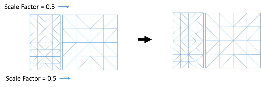
A solution (as adapted from [1]) is to assign “scale factors” to patch edges. First, the patch generation algorithm must guarantee that patch sizes decrease in size by half – meaning, a smaller patch that neighbors a larger patch will always be half the size of the larger patch. When a patch has an edge that is neighbor to a larger patch, that edge is assigned a scale factor of 0.5. This indicates that the assigned tessellation level should be cut in half so the vertices are aligned. Updating the tessellation factor occurs in the control shader (TCS), after the dynamic LOD algorithm has evaluated the edge.
The scale factor solution takes advantage of the fact that different tessellation levels can be applied to different edges of the patch. If only one edge is neighboring a larger patch size, then only that edge needs to be updated. To ensure that vertices align, tessellation levels are clamped to powers of two, and the fractional_even_spacing parameter in the evaluation shader is used (this makes sure that all tessellated segments are spaced evenly and symmetrically along an edge) [5].
Implementation
This part of the report will document some of my attempts at implementing the concepts discussed previously. The first approach I took was the simple uniform patch terrain approach. The second approach I tried was a non-uniform patch terrain using a quadtree.
Uniform Patch Implementation
The uniform patch approach is fairly straightforward to implement. One set of vertex data is created that will be used for each patch. The data set contains four vertices and their associated attributes, such as origin and color texture coordinates (not heightmap coordinates). The vertices form a simple quad that is 20 by 20 OpenGL units. This vertex data is loaded into a vertex buffer object and sent to the GPU. Each patch that is drawn reuses this same vertex data – the model/view/projection matrices are used to position each patch in the world accordingly. This is convenient because there is no need to have a large data set of vertices sent to the GPU and the data does not have to be sent to the GPU for each draw call.
A scene file specifies various parameters for the terrain, such as how many tiles (a tile is simply a grid of 8 by 8 patches) wide and long the terrain should be, what heightmaps to use, what textures to use, etc.
The key to applying the heightmap is making sure each patch has the appropriate texture coordinates to map their vertices to the heightmap. The following steps achieve this:
- Use the size and origin of the terrain to determine where the lower-left most vertex in the terrain is (if looking from a top-down view). This position is found in world-coordinates.
- Using this “lower-left” world coordinate, the “upper-right” most vertex in the terrain can be found using the width and length of terrain specified in the scene file. There is now a conceptual world-coordinate rectangle around the terrain.
- When a vertex is processed by the vertex shader, its world coordinate can be compared to the extents of the terrain to interpolate a (u,v) coordinate between (0,0) and (1,1) to be used as a texture coordinate for the heightmap.
For each patch that is drawn:
- The vertex shader determines the (u,v) coordinates at which to sample the heightmap for each vertex.
- The tessellation control shader calculates the tessellation levels for each edge using a dynamic level of detail algorithm.
- The tessellation evaluation shader samples the heightmap and offsets all vertices accordingly.
- The geometry shader calculates wireframe information.
- The fragment shader samples color textures to be applied to the mesh and renders the wireframe if enabled.
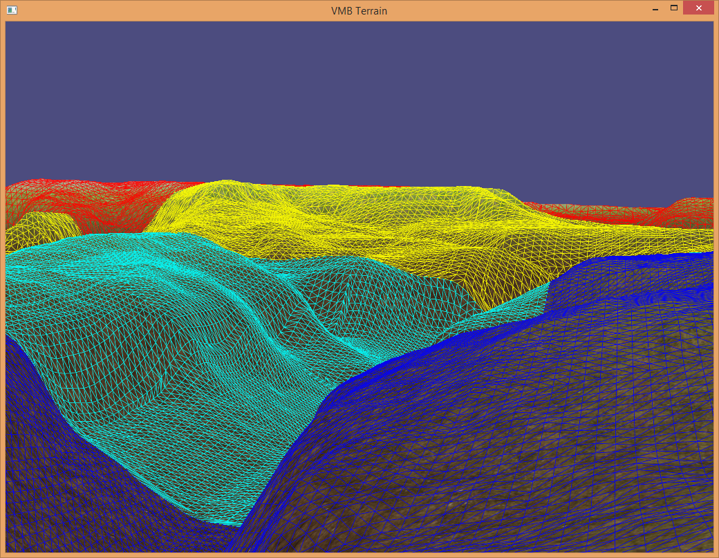
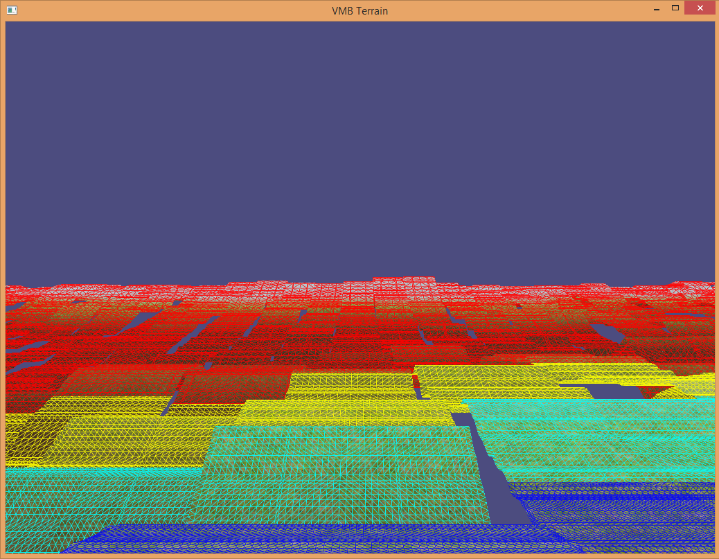
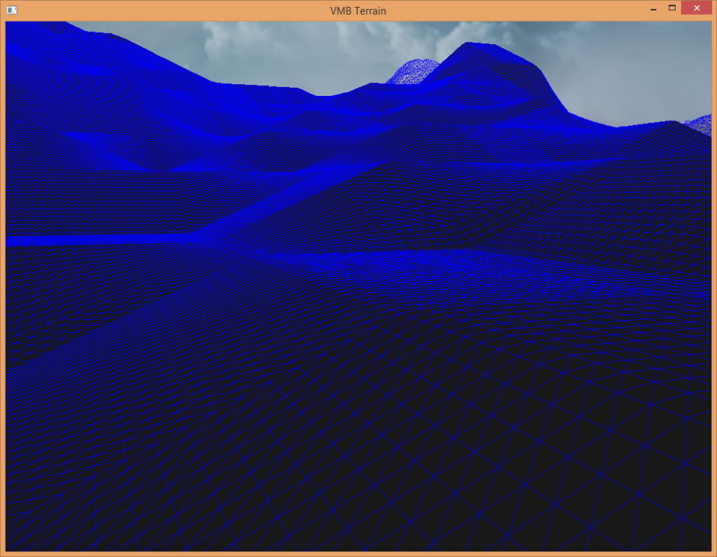
The sphere approach to dynamic level of detail was implemented for this approach, and it works very well. There are no cracking issues to deal with either. Figure 11 and Figure 13 show a terrain example with a wireframe overlay, which helps visualize the dynamic level of detail algorithm in action.
As mentioned previously, the uniform patch approach does not scale well – as terrains grow in size, performance decreases. This is when I turned to the non-uniform patch approach.
Non-Uniform Patch Implementation
A non-uniform patch terrain can lead to potentially better performance; however, it is much more involved to implement. The Frostbite™ 2 game engine from DICE uses a quadtree data structure for its terrain system (see [7] and [8] for details on this terrain system). For the quad tree, each successive layer in the tree represents a higher level of detail for a smaller patch size in the terrain. Each node in the tree tracks the origin, width, height and other parameters for the patch. The root of the tree represents the lowest level of detail, which would be a single patch covering the entire extent of the terrain.
For every frame, the terrain quadtree is recomputed to take into account where the camera is located in the world. The basic process for constructing the quadtree is as follows:
- Start with the root node. This is a single patch covering the entire terrain.
- Compare the position of the camera in the world to the origin of the node. If the camera is close enough to require additional levels of detail, subdivide the node into four smaller children.
- Repeat for each child node until a maximum subdivision level is reached, or the camera is far enough away that it doesn’t require any more subdivision for an acceptable level of detail.
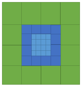
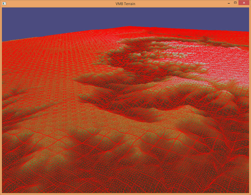
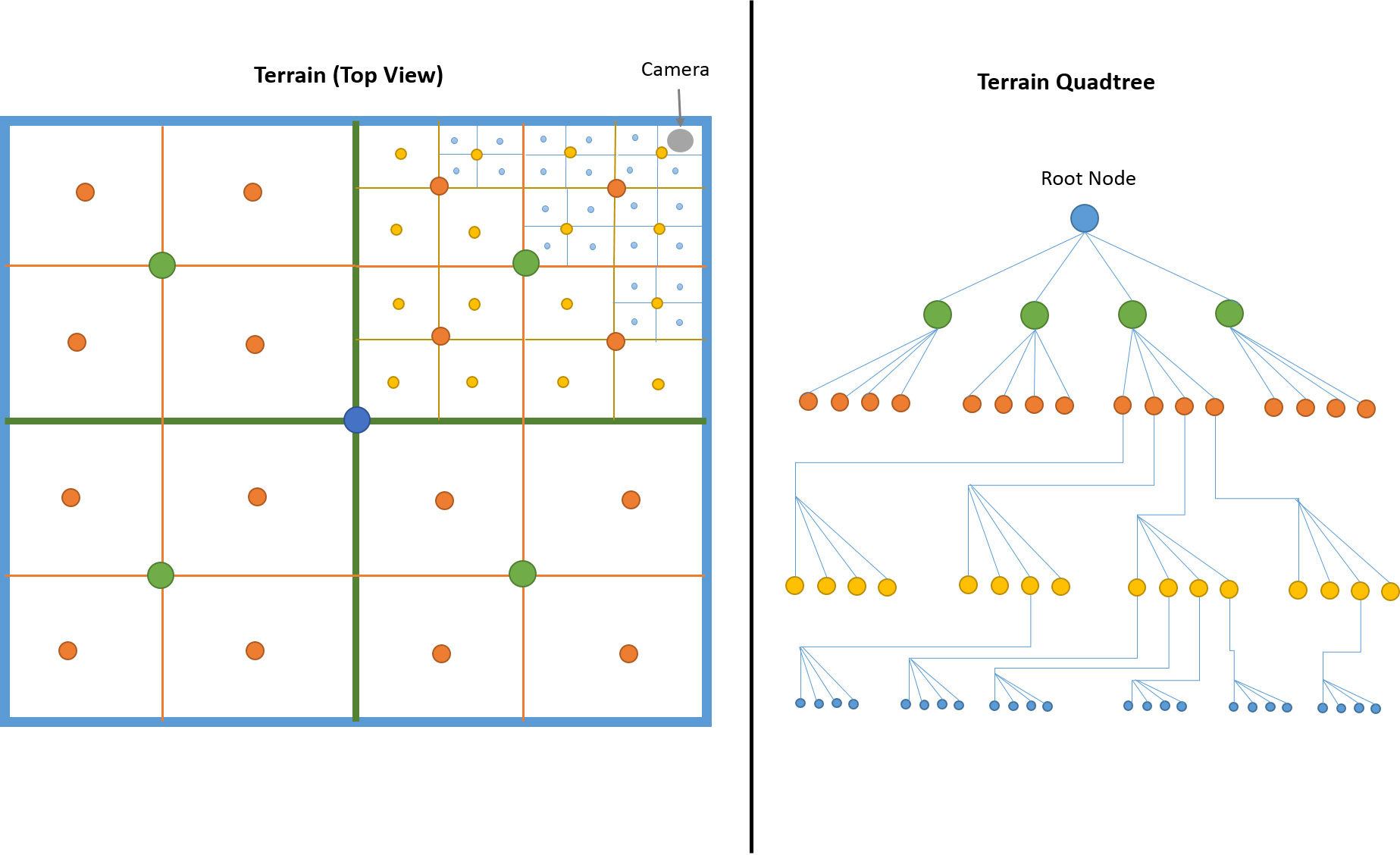
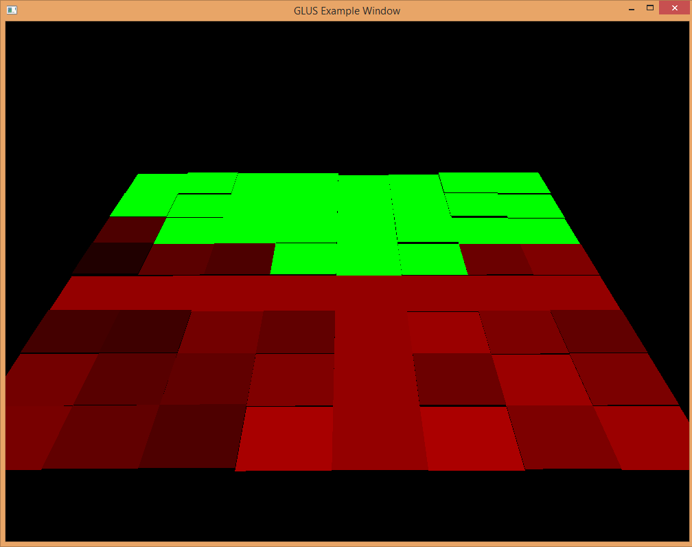
Figure 14 shows a visualization of a terrain that is subdivided into non-uniform size patches and the corresponding quadtree data structure. Note the camera position is in the upper-right corner of the terrain. The smaller sized patches are closest to the camera, and the patches grow in size as they get farther away.
Once the terrain quadtree is built, it can be traversed and the patches (nodes) that have no children are rendered (these are the nodes with the highest calculated level of detail, but smallest patch size). These patches can then be sent to the GPU to be tessellated and rendered.
Dealing with cracks for this approach was, by far, the most challenging part of implementation. As mentioned before, a tessellation scale factor is applied to each edge of a patch before it is rendered. Although it seems simple at first, tracking whether or not a neighboring patch has/will be subdivided can be difficult. I found the easiest way to assign scale factors for edges was to do it after the entire quadtree is computed and right before a patch is rendered. Before a node is rendered, a search is made through the tree for its four neighbors (north, south, east, west). The size of each neighbor is compared to the node, and a scale factor can be appropriately applied to each edge. In the tessellation control shader, after the dynamic level of detail algorithm computes a tessellation level for an edge, the scale factor can be applied.
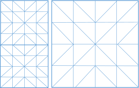
Initially, the sphere approach to dynamic LOD was applied (just as in the uniform patch approach previously). However, I still had cracking issues with this algorithm. I finally reverted to the camera distance approach for dynamic LOD, which fixed the cracking issue. I have yet to figure out why this is. Figure 20 and Figure 21 are a comparison of the two algorithms in action.
Other Technical Challenges
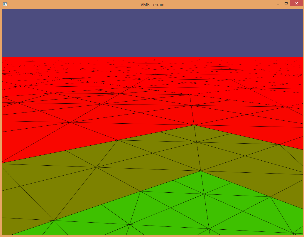
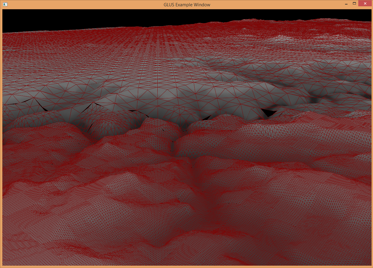
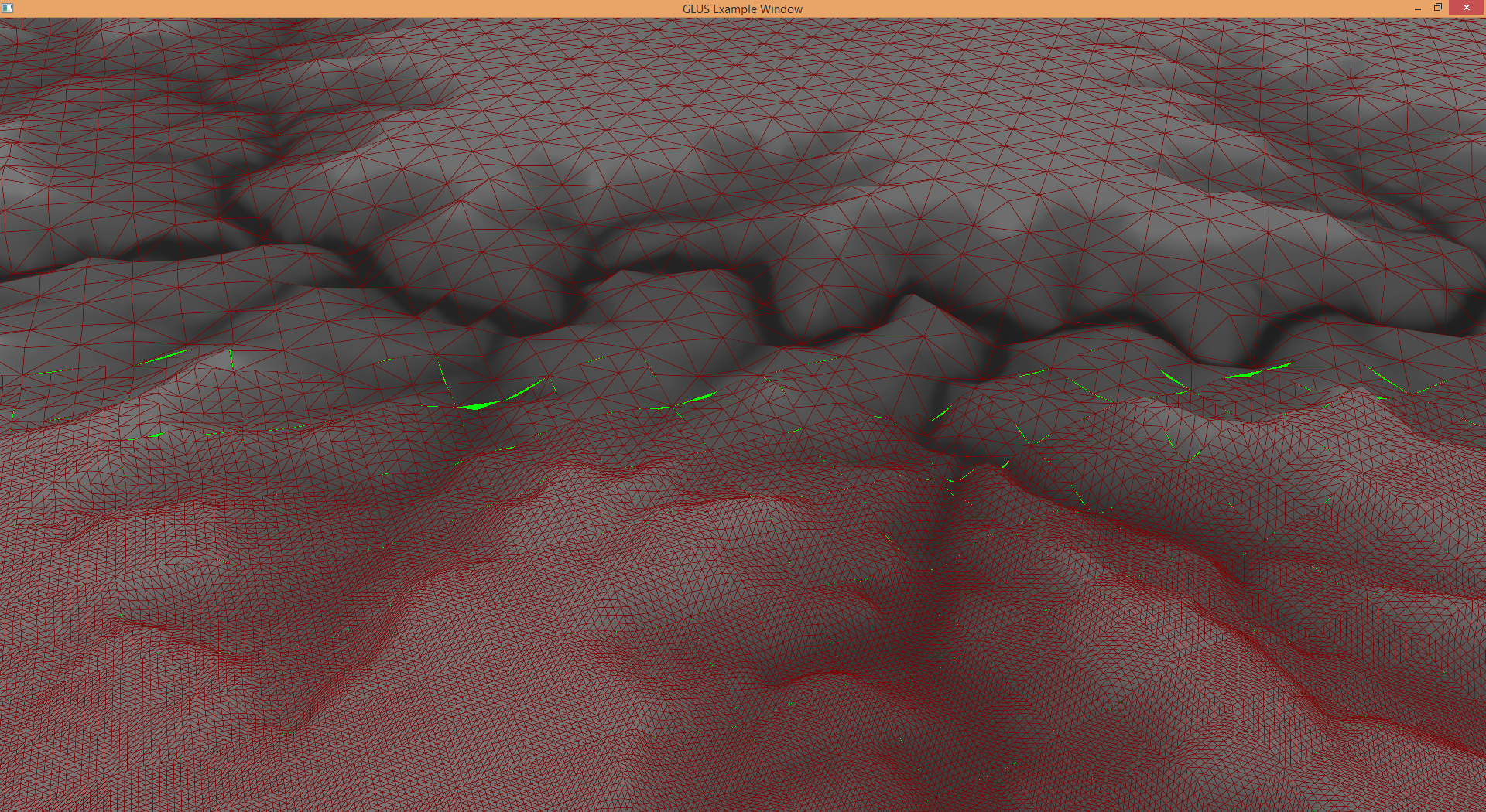
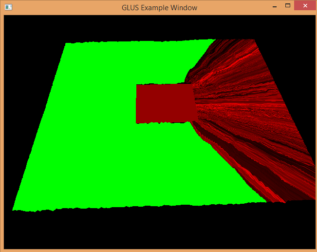
GPU debugging can be quite difficult compared to modern CPU debugging. Tools like gDebugger (http://www.gremedy.com) are very helpful in providing information; however, sometimes other approaches must be taken to narrow down what is wrong. One thing I did frequently was use the fragment shader to check the value of certain variables or parameters I was having concern with and assign different colors to certain fragments depending on the variable’s value. This can help provide some insight into certain situations. Figure 22 and Figure 23 demonstrate this.
Terrain Cracks
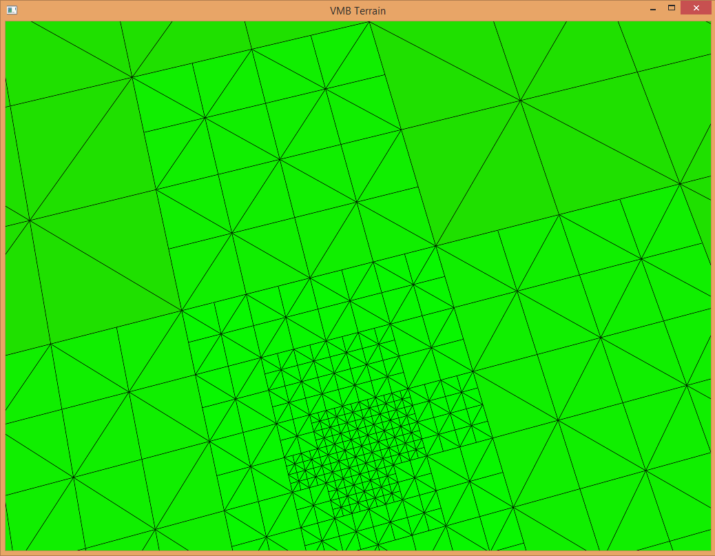
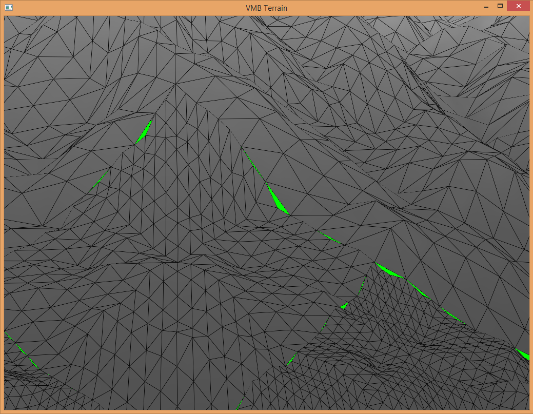
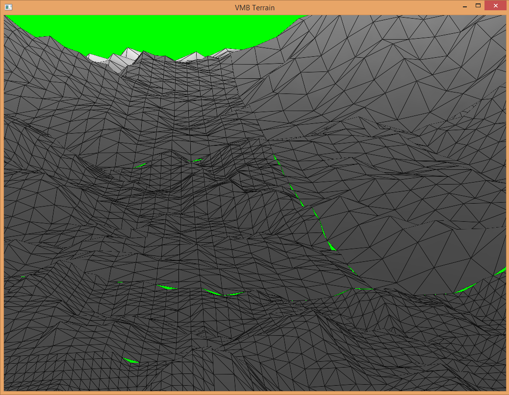
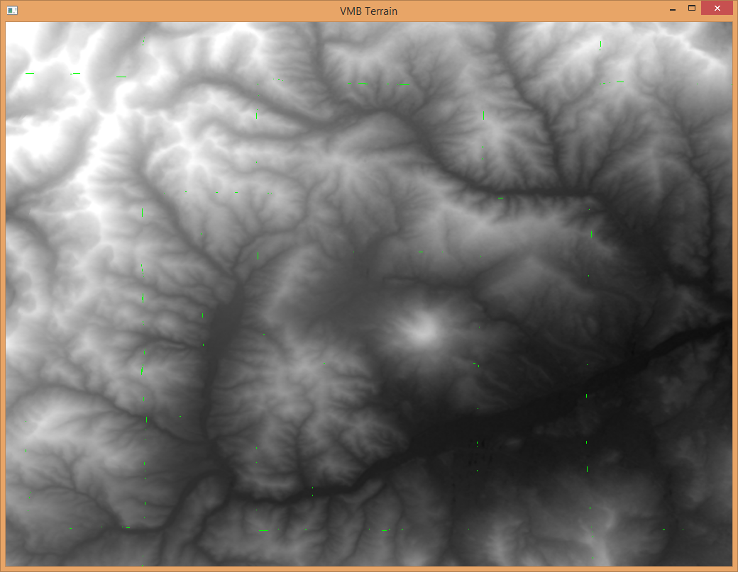
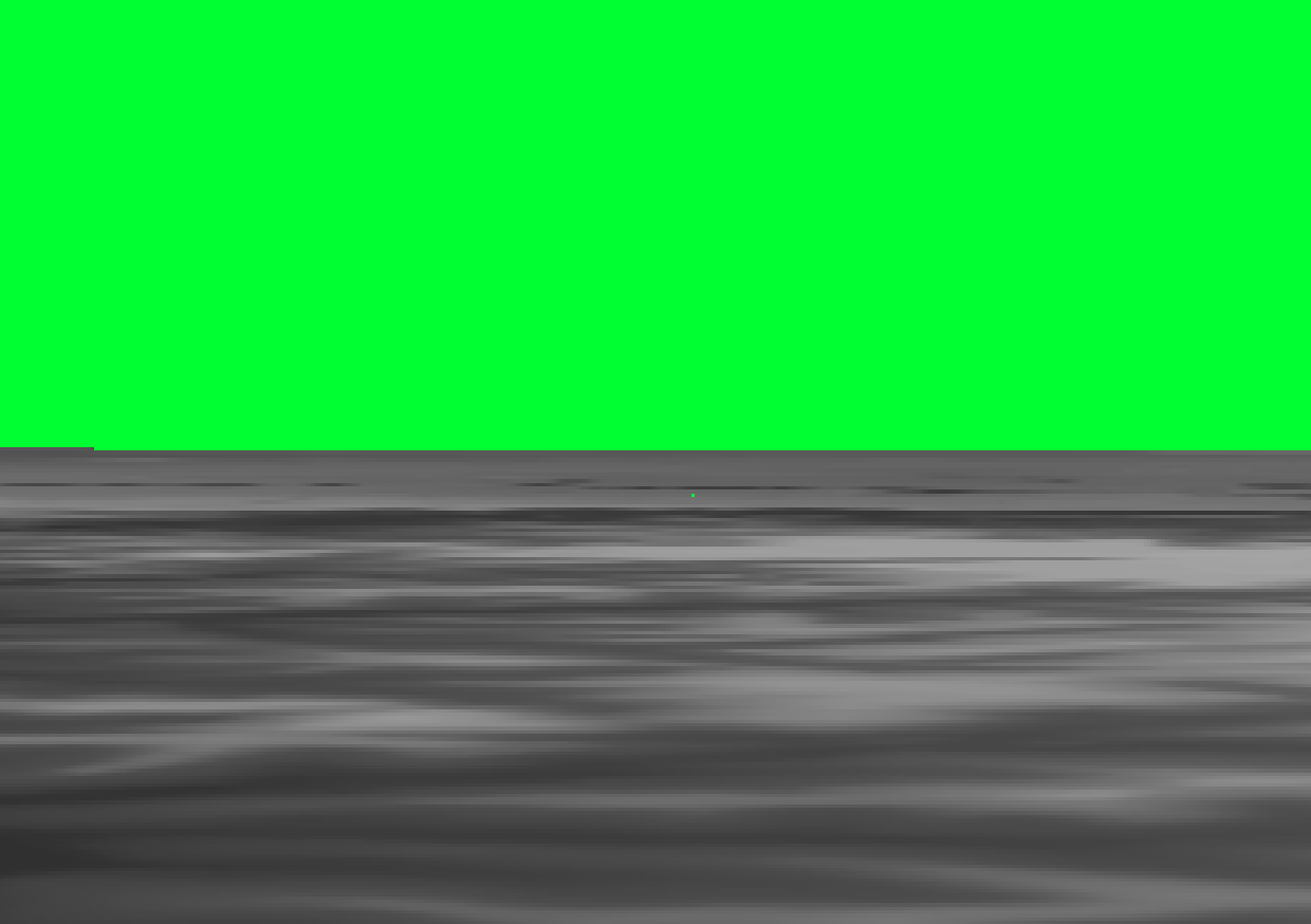
When debugging cracks in a terrain, it is helpful to have a very bright contrast color as the background to help identify cracks. Lime green works well in a lot of situations.
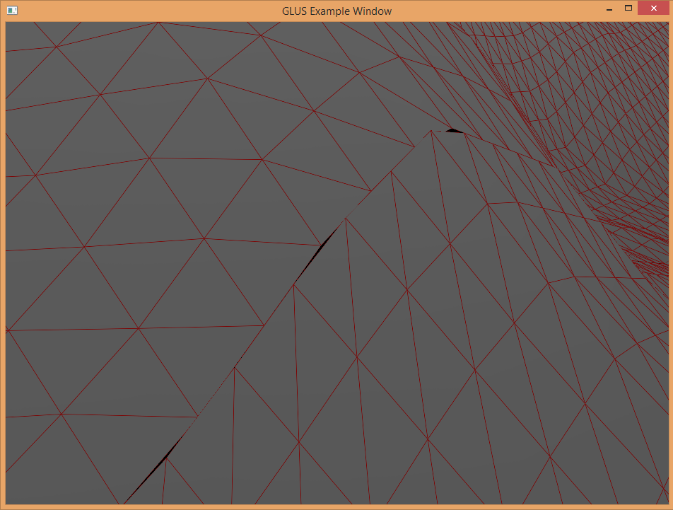
While dealing with cracks, I had a separate, puzzling issue. Sometimes I would have very small, one pixel cracks appear (when dealing with the uniform-patch terrain). My guess is some kind of rounding issue, but I was not able to confirm this. Figure 24 is a zoomed-in screenshot showing a single pixel crack.
Uniform Buffer Objects
In newer versions of OpenGL, a uniform buffer object (UBO) can be created to allow multiple OpenGL programs to share uniform data. For example, a model-view-projection matrix could be calculated for the scene, sent to the GPU, put into the uniform buffer object, and used by two different programs.
When using this technique, I would sometimes receive random results with no discernable cause. Sometimes I could remove the UBO, recompile, then add the UBO back in, recompile and things would go back to normal. This was definitely the most puzzling issue in the whole project. It wasn’t a show-stopper by any means, however. I simply had to stop using the UBO and update the matrix information the “old-fashion” way. Figure 25 and Figure 26 highlight these odd results.
Possibilities for Future Work
Multiple heightmaps
The current (non-uniform) implementation of the project uses a single heightmap for the entire terrain. For large terrains, the heightmap must be a very high resolution to provide accurate sampling for high level of details (i.e. when the camera is very close to the terrain). The quadtree data structure provides a mechanism so multiple heightmaps can be used. A higher-detail heightmap can be assigned to nodes at a higher level-of-detail and a coarser one for lower level-of-detail nodes.
Real-world GIS data
It would be possible to read real world terrain data from sources like digital elevation models (DEMs) and LIDAR data sets. For this project, heightmaps were extracted from DEMs while disregarding any scale or coordinate data. LIDAR data sets were considered, but for simplicity sake were not used.
Additional features
Many additional features could be added, such as lighting and shading, texturing, models, decals, roads, environmental effects, etc. The quadtree structure would allow these features to also scale with a dynamic level-of-detail as well.
Miscellaneous Project Notes
- GLUS (Graphic Library UtilitieS) was used for this project instead of GLUT. It has functions for loading and compiling shader programs, image loading functions for TGA images, various matrix and vector manipulation functions, and more.
- The “grand_canyon_xxx” image files are from the GLUS example projects.
- The US Geological Survey (USGS) Web site (http://earthexplorer.usgs.gov) was used to source some digital elevation models for heightmaps.
- A program called QGIS (http://qgis.org) was used to extract heightmaps from these DEMs.
- Basic texture splatting was implemented in the uniform-patch implementation. Some details about texture splatting can be found at (http://www.cbloom.com/3d/techdocs/splatting.txt).
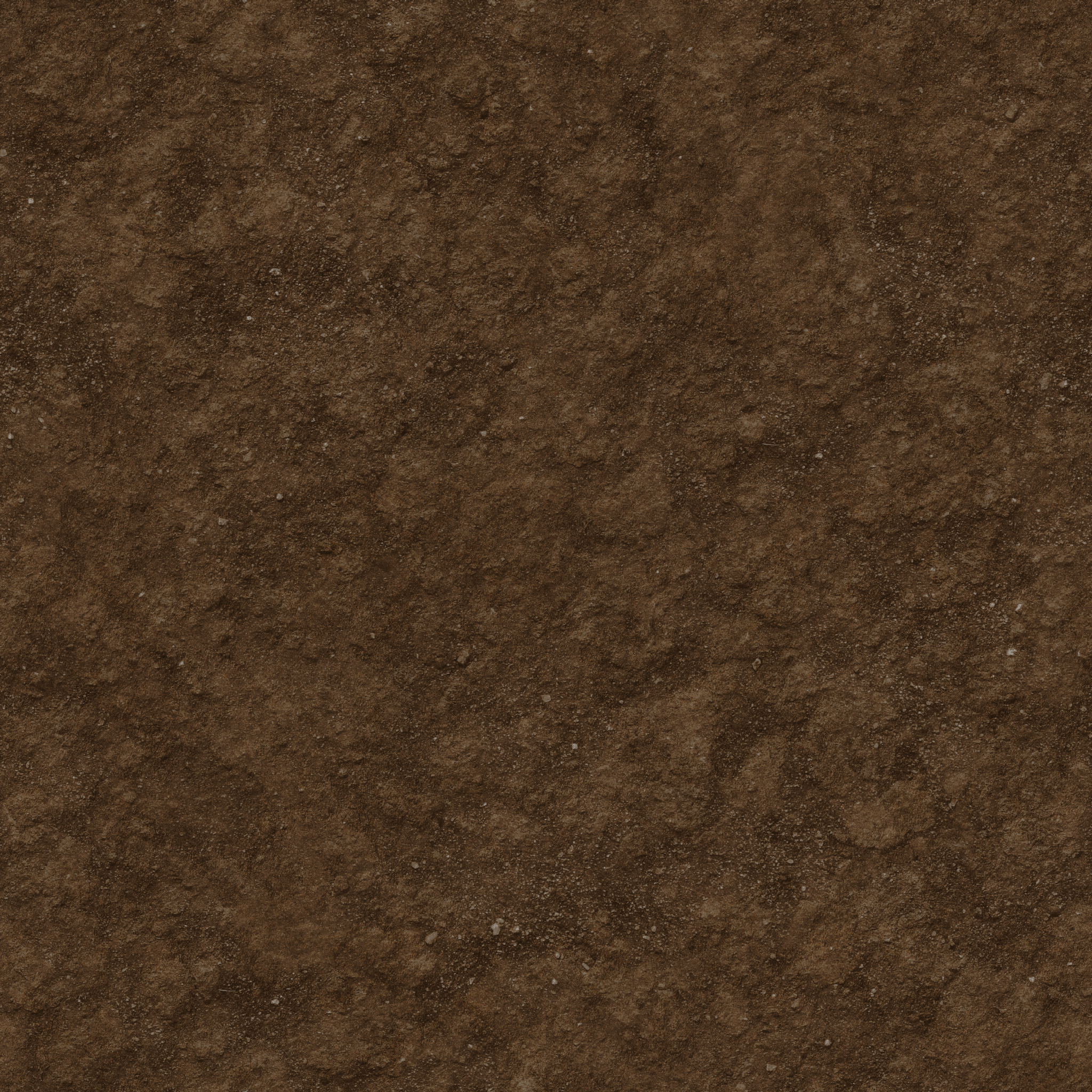
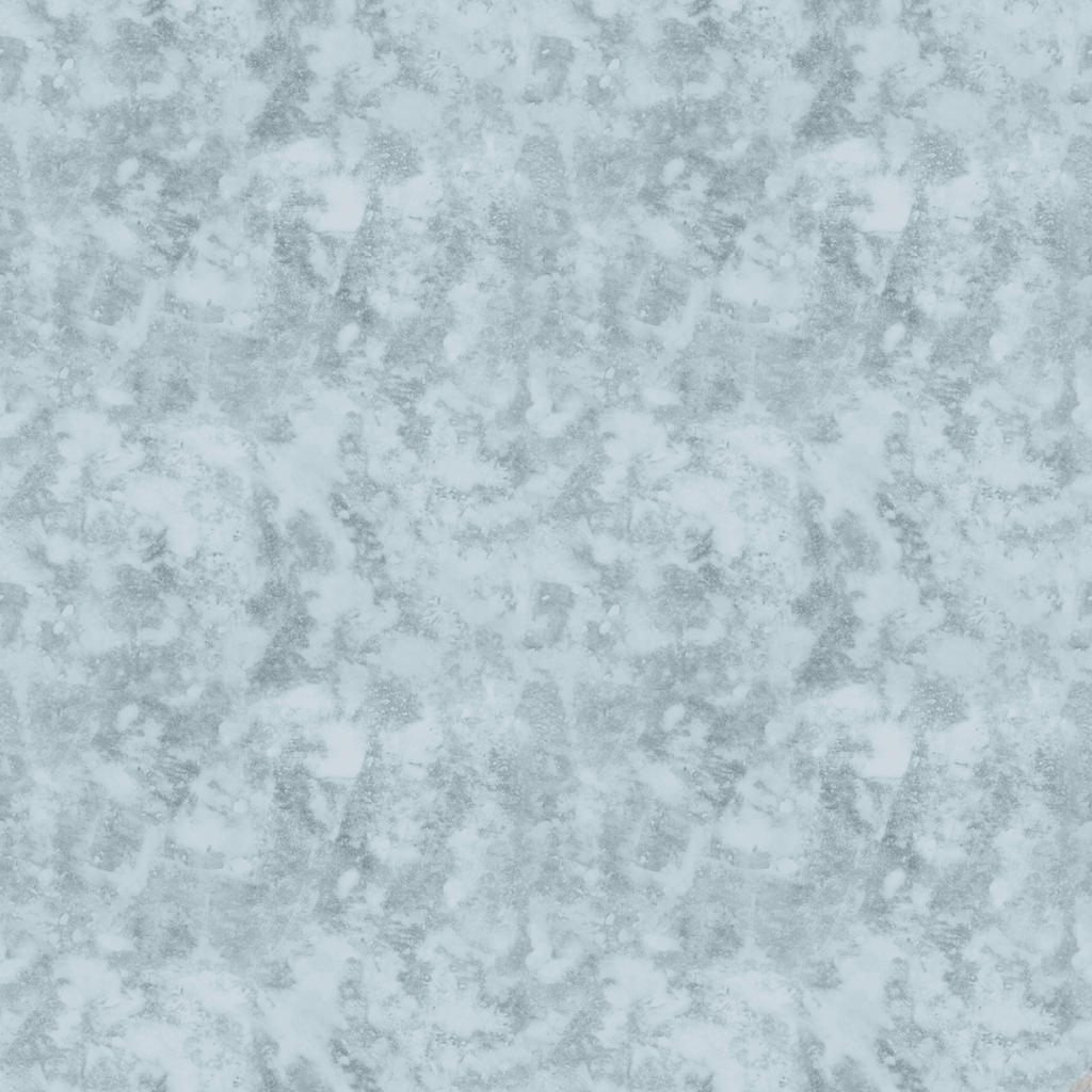
- Texture sources:
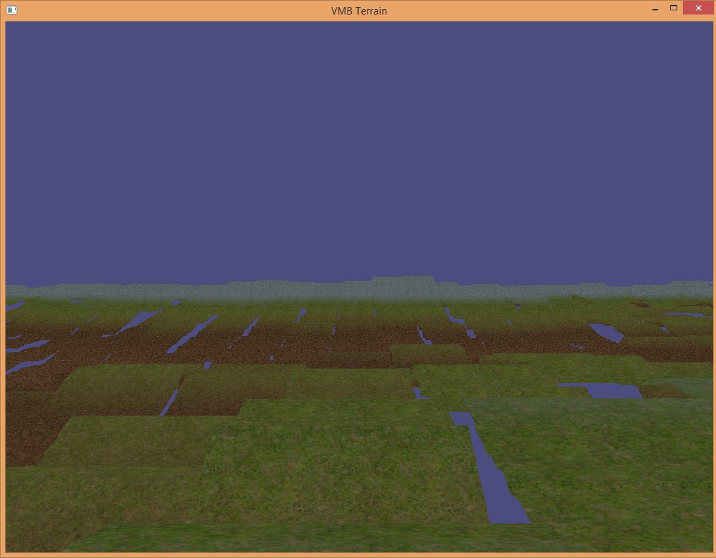
- A skybox was implemented in the non-uniform patch implementation. The textures for the skybox were made by Jockum Skoglund (also known by alias “hipshot”). His Web site can be found at zfight.com.
Conclusion
This project covered quite a bit of ground for someone with limited experience with OpenGL. I now have a better understanding of OpenGL 4.x, shaders and GLSL, vertex buffer objects, vertex attribute arrays, tessellation, and much more, in addition to the terrain rendering techniques explored.
References
[1] I. Cantlay, “DirectX 11 Terrain Tessellation,” NVIDIA, 2011.
[2] D. Wolff, OpenGL 4 Shading Language Cookbook, Birmingham B3 2PB, UK: Packt Publishing Ltd., 2013.
[3] OpenGL Wiki, “Rendering Pipeline Overview,” OpenGL, [Online]. Available: https://www.opengl.org/wiki/Rendering_Pipeline_Overview.
[4] OpenGL Wiki, “Tessellation Control Shader,” [Online]. Available: https://www.opengl.org/wiki/Tessellation_Control_Shader.
[6] OpenGL Wiki, “Tessellation,” [Online].
[7] A. Cervin, “Adaptive Hardware-accelerated Terrain Tessellation,” Linkoping University, Norrkoping, Sweden, 2012.
[8] M. Widmark, “Terrain in Battlefield 3: A modern, complete and scalable system,” in Game Developers Conference 2012, San Francisco, CA, 2012.
[9] C. Bloom, “Terrain Texture Compositing by Blending in the Frame-Buffer,” 2000.